R中媲美Python Dictionary的神器-hash

在Python中有这样一个神通广大的数据类型，它叫Dictionary。而长久以来在R中想要实现类似的Hash存储只能依靠environment类型，用起来非常不友好。

今天很偶然的发现了一个新的R包（其实也不新了，09年就已经发布，竟然一直没有发现）hash，它对environment进行了封装，使用户可以很方便的利用Hash表进行存储。

详细用法见文档

其中有几个地方需要特别注意的：

1. Hash表的Key必须为字符类型的，而且不能是空字符串""

2. 引用传递。在R中environment和hash对象只存在一份全局拷贝，因此如果在函数内改变它的值将会影响到外部访问的结果。如果需要复制hash对象，需调用它的copy方法。

3. 内存释放。通过rm销毁hash对象时，其占用的内存不会自动释放，因此需在rm前调用clear，以防内存泄露。

性能比较

hash对象的性能自然是没得说，下图是和list的一些比较。

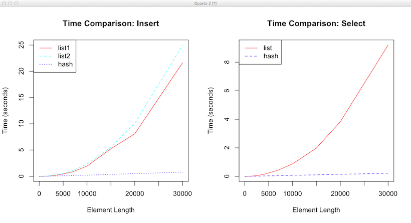
左图是连续插入数据的时间，list1和list2分别表示两种向list中插入数据的方法；右图是通过指定Key的方式遍历整个对象所需的时间。从图中很明显的可以看到采用list对象无论是插入还是查找，性能随数据规模的增加下降非常明显。而hash对象的性能受数据规模影响非常小，近乎常数时间。

代码

见这里或者往下看。

# Encoding: utf8
library(hash)

list1.insert.test <- function(len) {
    a <- list()
    res <- system.time({
        for(i in 1:len)
            a[[as.character(i)]] <- i
    })
    res[3]
}

list2.insert.test <- function(len) {
    a <- list()
    res <- system.time({
        for(i in 1:len)
            a <- c(a,i)
        names(a) <- 1:len
    })
    res[3]
}

hash.insert.test <- function(len) {
    a <- hash()
    res <- system.time({
        for(i in 1:len)
            a[[as.character(i)]] <- i
    })
    clear(a)
    res[3]
}

list.select.test <- function(len) {
    a <- hash(1:len,1:len)
    b <- as.list(a)
    clear(a)
    x <- names(b)
    res <- system.time({ invisible(sapply(x,
            function(i) {
                b[[i]]
            }))
    })
    res[3]
}

hash.select.test <- function(len) {
    a <- hash(1:len,1:len)
    x <- keys(a)
    res <- system.time({ invisible(sapply(x,
            function(i) {
                a[[i]]
            }))
    })
    clear(a)
    res[3]
}

run.test <- function(fun, x, .progress='text') {
    require(plyr)
    laply(x,fun,.progress=.progress)
}

### ------ Main ------
x <- c(10,100,200,300,400,500,600,800,1000,1500,
        2000,3000,4000,5000,7000,10000,15000,20000,30000)
list1.insert.time <- run.test(list1.insert.test, x)
list2.insert.time <- run.test(list2.insert.test, x)
hash.insert.time <- run.test(hash.insert.test, x)
p <- par(mfrow=c(1,2))
plot(x, list1.insert.time, type='l', 
     col='red',lty=1,
     ylim=range(c(list1.insert.time,list2.insert.time,hash.insert.time)),
     main='Time Comparison: Insert',
     xlab='Element Length',ylab='Time (seconds)')
lines(x, list2.insert.time, col='cyan', lty=2)
lines(x, hash.insert.time, col='blue', lty=3)
legend('topleft', c('list1','list2','hash'), col=c('red','cyan','blue'), lty=c(1,2,3))

list.select.time <- run.test(list.select.test, x)
hash.select.time <- run.test(hash.select.test, x)
plot(x, list.select.time, type='l',
     col='red',lty=1,
     ylim=range(c(list.select.time,hash.select.time)),
     main='Time Comparison: Select',
     xlab='Element Length',ylab='Time (seconds)')
lines(x, hash.select.time, col='blue', lty=2)
legend('topleft', c('list','hash'), col=c('red','blue'), lty=c(1,2))
par(p)